Mathematical analysis of a predator-prey system with shared resource, climatic effects, and neural network insight

This research paper introduces a predator-prey system in which both organisms depend on a common sustenance source. In order to establish environmental dynamics that are more plausible, we integrated climatic effects on the predator population by implementing a sigmoidal function. The objective is to study the impact of climate on the population dynamics of interacting species by employing mathematical tools like stability analysis and Artificial Neural Networks. By employing meticulous mathematical analysis, we were able to ascertain the equilibrium points of the system and examine their stability on a global scale. Our investigation covered both diffusive and non-diffusive models, providing insight into the unique dynamical characteristics of each. Moreover, in order to leverage the capabilities of modern computational methods, a neural network strategy was implemented to analyses the system's complexities in greater detail. In conclusion, exhaustive diagrams were used to meticulously illustrate the effect of varying parameters, thereby providing invaluable insights into the behavior of the system under various conditions.

Introduction

The concept of prey-predator communication was first presented by Lotka (1925) and Volterra (1926) [1] in their groundbreaking research. Holling [2] further expanded on this concept by developing prey-predator models that included three different types of functional responses to explain the dynamics of predation. These models of biological interest are developed using nonlinear systems, which are represented by ordinary and partial differential equations. The mathematical model of prey-predator dynamics is influenced by the prey-predator mathematical model derived from the coexistence of foxes and rabbits. Foxes prey on rabbits, while rabbits consume clover. The safety of rabbits will rise as the population of foxes drops, and conversely, if the rabbit population declines, the fox population will grow [3]. The population dynamics of the two kinds of animals, characterized by declining and growing trends, are modeled using ordinary differential equations for a nonlinear prey-predator system. The relationship between predators and their prey has a rich historical background and will persist as a fundamental concept in mathematical ecology due to its global importance and inherent truth [4]. Mathematical biology frequently involves the utilization of both modelling and simulations. Biological structures are commonly depicted using systems of nonlinear Ordinary Differential Equations (ODEs). Nonlinear Ordinary Differential Equation (ODE) models are frequently distinguished by their inherent challenge in determining solutions. These objects are typically categorised as rigid or impractical and are recognised for presenting substantial difficulties and intricacies when trying to find analytical solutions. Therefore, the very efficient and powerful approach for finding numerical solutions to these nonlinear systems has attracted considerable attention. The predominant focus of the research community has been on prey-predator models that involve interactions between two variables, namely interspecific interactions. However, Danca, et al. [5], Jing, et al. [6], Liu, et al. [7], and Elabbasy, et al. [8] have published work on discrete-time nonlinear models of prey-predator dynamics. The durability of the dynamics in discrete-time models surpasses that of continuous-time systems in terms of longevity. Summers, et al. conducted research on four discrete-time ecosystem models that were influenced by periodic forcing effects [9]. In a separate study, Danca, et al. collaborated with Holling to examine the chaotic dynamics of discrete-time prey-predator systems [5]. In recent times, several novel techniques have been developed to effectively address these types of nonlinear issues. Some examples of methods used in this study include the Runge-Kutta-Fehlberg method, the Laplace Adomian decomposition method [10], the differential transformation method [11], the finite element method [12], the Sumudu decomposition method [13], the Homotopy analysis method [14], the new coupled fractional reduced differential transform method [15], and the confidence. There are pros and cons to each of these predictable methods. On the other hand, bio-inspired and nature-inspired heuristics-based stochastic solvers have not yet been used to solve nonlinear systems that describe prey-predator models. In [16] global stability of the diffusive and non-diffusive predator-prey model is discussed in which common food is considered for both species. In [17,18] authors have presented three species of predator-prey systems taking the common food by predator and a prey species and disease in the interacting species. In [19] fractional-order predator-prey model is presented and analysed.

Stochastic computing paradigms that use artificial intelligence algorithms have been successfully implemented to solve linear and nonlinear models in many applications within the fields of applied science and technology [20,21]. Some notable recent applications of stochastic solvers include solving nonlinear system models for electrical conducting solids [22], representing atomic physics models using the Thomas-Fermi equation [23], modelling fuzzy-type nonlinear differential equations [24], studying combustion theory models for fuel ignition [25], and analysing nonlinear Navier-Stokes systems [26]. Nonlinear systems of pantograph delay differential equations [27], Volterra integral systems [28,29], nanofluids models of mechanics [30], Fredholm integral equations [31], the spherical cloud of gas model [32], astronomy models of Flierl–Petviashivili type [33], control systems of fractional order [34], bilinear programming models [35], nonlinear Jeffery–Hamel flow containing nanoparticles [36], and nonlinear Bratu models [37]. These facts not only highlight the importance of stochastic solvers in various applications, but also provide motivation for authors to conduct exploration and exploitation in order to develop a precise, dependable, resilient, stable, and efficient computing paradigm for nonlinear prey-predator problems.

This study explores the predator-prey model, examining the impact of climate on species interactions. It uses neural networking techniques to predict future scenarios, enhancing our understanding of ecological systems and contributing to artificial neural networking techniques. The study integrates climate variables into the predator-prey framework, revealing a more comprehensive understanding of species balance in the face of environmental changes. The main aim of this research is to investigate the climatic effects along with future predictions about the behavior of the model by using ANN. The visual representation of results through plots captivates the scientific community and opens up new explorations.

The setting of this paper is presented ahead. The second section deals with the modeling of the predator-prey system. The third section deals with the equilibrium points of the model along with the stability of a non-diffusive system. The fourth section deals with the stability self-diffusive system. Simulations are presented in section five. In sections (6) and (7) discussion and conclusion are presented.

The model

The interaction between species in predator-prey modeling is greatly affected by environmental factors such as the availability of food, water, shelter, and many more to name a few. It has been observed that climatic factors are crucial in this regard. Climate changes are affecting the population throughout the globe. We consider a predator-prey model in which predator and prey depend on a common food resource and predators are being affected by the environmental changes. This system is an extension of the system presented in [16], in which two species relying on a common food were considered. We define the following system of Ordinary Differential Equations (ODEs):

$\frac{\text{dP}}{\text{dt}}=P\left(-m+\frac{af}{bN+aP}+N\alpha -\frac{k}{1+{\text{e}}^{-\frac{\text{δT}}{\sigma }}}\right)\text{ (1)}$

$\frac{\text{dN}}{\text{dt}}=N\left(-n+\frac{bf}{bN+aP}-P\alpha \right)\text{ (2)}$

Where P and N are respectively the functions of predator and prey. Here f shows the common resource and a, b are consumption rates of food by predator and prey, respectively. The predation rate is α, the temperature-dependent term $\frac{k}{1+{\text{e}}^{-\frac{\text{δT}}{\sigma }}}$ introduces a sigmoidal response to temperature changes, influencing the predator population. A further breakdown of the involved parameters is given next. k Displays the sensitivity of the predator population to temperature changes, 𝛿T, and 𝜎 respectively show the difference between the current temperature and reference temperature and width parameter of the sigmoidal temperature response.

Stability analysis for non-diffusive system

In this section, we present the equilibrium points of the model and the analysis of the fixed points for the global stability of coexistence fixed points.

To find the equilibrium points we solve the following system of equations

$P\left(-m+\frac{af}{bN+aP}+N\alpha -\frac{k}{1+{\text{e}}^{-\frac{\text{δT}}{\sigma }}}\right)=0\text{ (4)}$

$N\left(-n+\frac{bf}{bN+aP}-P\alpha \right)=0\text{ (4)}$

The solution of the above system leads to the following result.

$E_1=\left(0,\frac{f}{n}\right),\text{ (5)}$

${\text{E}}_2=\left(\frac{\left(1+e^{\frac{\text{δT}}{\sigma }}\right)f}{m+e^{\frac{\text{δT}}{\sigma }}\left(k+m\right)},0\right),\text{ (6)}$

$E_3(P^{*},N^{*})=\left(\begin{array}{c}\frac{-bmn+a{n}^2+bf\alpha +e^{\frac{\text{δT}}{\sigma }}\left(-b\left(k+m\right)n+a{n}^2+bf\alpha \right)}{\left(bm-an+e^{\frac{\text{δT}}{\sigma }}\left(b\left(k+m\right)-an\right)\right)\alpha },\\ \frac{b{(m+e^{\text{δT}/\sigma }(k+m))}^2-a(1+e^{\text{δT}/\sigma })(mn+f\alpha +e^{\text{δT}/\sigma }((k+m)n+f\alpha ))}{(1+e^{\text{δT}/\sigma })(bm-an+e^{\text{δT}/\sigma }(b(k+m)-an))\alpha }\end{array}\right)\text{ (7)}$

$\phi =\left\{\left(P^{*},N^{*}\right); P^{*}>0,N^{*}>0\right\}\text{ (8)}$

Theorem.1 Suppose the inequalities hold for positive parameters of the model (1)-(3), then (P*, N*) is Lyapunov stable in φ.

Proof: We consider the Lyapunov function [16] given below

$L(P,N)={\displaystyle {\int }_{P^{\text{*}}}^P\frac{ϵ-P}{ϵ}}\text{ d}ϵ+{\displaystyle {\int }_{\text{N}}^{\text{N}}\frac{\xi -N}{\xi }}\text{ d}\xi \text{ (9)}$

The derivative of (9) leads to the following

$\stackrel{\cdot }{{\displaystyle L}}=\stackrel{\cdot }{{\displaystyle \text{P}}}\frac{(P-P^{\text{*}})}{P}+\stackrel{\cdot }{{\displaystyle N}}\frac{(\text{N}-{\text{N}}^{\text{*}})}{\text{N}}\text{ (10)}$

As (P*, N*) is an equilibrium point, we have

$\dot{L}=\left(P-P^{\text{*}}\right)\left(\frac{af}{bN+aP}+N\alpha -\frac{af}{b{N}^{*}+a{P}^{*}}-N^{*}\alpha \right)+(\text{N}-{\text{N}}^{\text{*}})\left(\frac{bf}{bN+aP}-P\alpha -\frac{bf}{b{N}^{*}+a{P}^{*}}+P^{*}\alpha \right)$

We further simplify the above equation

$\dot{L}=\left(P-P^{\text{*}}\right)\left(\frac{af\left(b{N}^{*}+a{P}^{*}\right)-af\left(aP+bN\right)+\alpha \left(\text{N}-{\text{N}}^{\text{*}}\right)\left(bN+aP\right)\left(b{N}^{*}+a{P}^{*}\right)}{\left(bN+aP\right)\left(b{N}^{*}+a{P}^{*}\right)}\right)+$

$(\text{N}-{\text{N}}^{\text{*}})\left(\frac{bf\left(b{N}^{*}+a{P}^{*}\right)-bf\left(aP+bN\right)-\alpha \left(\text{P}-{\text{P}}^{\text{*}}\right)\left(bN+aP\right)\left(b{N}^{*}+a{P}^{*}\right)}{\left(bN+aP\right)\left(b{N}^{*}+a{P}^{*}\right)}\right)$

Some more simplifications lead to the following

$\dot{L}=-f\frac{{[(aP+b\text{N})-(a{P}^{\text{*}}+b{\text{N}}^{\text{*}})]}^2}{\left(bN+aP\right)\left(b{N}^{*}+a{P}^{*}\right)}\le 0\text{ (11)}$

Which proves the Lyapunov stability.

Stability analysis for the diffusive system

Within the dynamical population model, habitat structure is influenced by random walks, with species movement dictated by environmental factors such as food resources and protection. The stochastic nature of this movement exhibits variation across locations due to the diverse environmental conditions. Furthermore, the density of species within their habitats demonstrates variability.

The following section deals with the implications of diffusion on the coexistence of species.

The self-diffusion system for (1-2) can be written as

$\frac{\partial \text{P}(\text{x},\text{t})}{dt}=d_{11}△P+P\left(-m+\frac{af}{bN+aP}+N\alpha -\frac{k}{1+{\text{e}}^{-\frac{\text{δT}}{\sigma }}}\right),xϵ \Omega ,t>0\text{ (12)}$

$\frac{\partial \text{N}(\text{x},\text{t})}{dt}=d_{22}△N+N\left(-n+\frac{bf}{bN+aP}-P\alpha \right),\text{ x}ϵ \Omega ,\text{ t}>0\text{ (13)}$

Where, $\frac{\partial \text{P}}{\partial \vartheta }=\frac{\partial \text{N}}{\partial \vartheta }=0,\text{ x}ϵ \partial \Omega ,\text{ t}>0\text{ (14)}$

In the provided mathematical framework, P(x,t) and N(x,t) represent the respective population densities of predators and prey at a designated location x within the defined domain at time t. The domain Ω possesses a smooth boundary denoted as ∂Ω, and ϑ signifies the outward unit normal vector on this boundary.

The Neumann boundary conditions stipulate that there is no population flux across the boundary. This condition enforces a balance at the edges of the domain, ensuring that the population dynamics of both predators and prey are subject to equilibrium or stability at the boundary. The initial condition is as under

${\Phi }_0=\{\text{P}(\text{x},0)=P_0(\text{x})\ge 0,\text{N}(\text{x},0)=N_0(\text{x})\ge 0\}\text{ (15)}$

Here d₁₁, d₂₂, are non-negative self-diffusion parameters. The solution to the above system has global existence and boundedness, according to Hollis results.

Theorem 2 Let Ω be a bounded domain with smooth boundary ∂Ω. Suppose a, b, d₁₁, d₂₂ and f be positive and (19) holds then (P*, N*) of (12-13) is Lyapunov stable in

$\omega =\{\left(P,N\right),P>0,N>0\}.$

Proof. It is obvious that {(P, N), P = 0}, {(P, N), N = 0} are the invariant manifolds. We establish the Lyapunov function to determine the stability of the self-diffusive system as shown below

$ℒ(P,\text{N})=\underset{\text{Ω}}{{\displaystyle \int }}\underset{P^{\text{*}}}{\overset{P}{{\displaystyle \int }}}\frac{ϵ-P^{\text{*}}}{ϵ}dϵdX+\underset{\text{Ω}}{{\displaystyle \int }}\underset{{\text{N}}^{\text{*}}}{\overset{\text{N}}{{\displaystyle \int }}}\frac{\xi -{\text{N}}^{\text{*}}}{\xi }d\xi dX\text{ (16)}$

Now taking derivative with respect to “t” on both sides, we get

$\frac{dℒ}{dt}={{\displaystyle \int }}_{\text{Ω}}\frac{\text{P}-{\text{P}}^{\text{*}}}{\text{P}}\frac{\partial \text{P}}{dt}dX+{{\displaystyle \int }}_{\text{Ω}}\frac{\text{N}-{\text{N}}^{\text{*}}}{\text{N}}\frac{\partial \text{N}}{dt}dX\text{ (17)}$

$\begin{array}{l}\frac{dℒ}{dt}={{\displaystyle \int }}_{\text{Ω}}\frac{\text{P}-{\text{P}}^{\text{*}}}{\text{P}}\left[d_{11}△P+P\left(-m+\frac{af}{bN+aP}+N\alpha -\frac{k}{1+{\text{e}}^{-\frac{\text{δT}}{\sigma }}}\right)\right]dX\\ +{{\displaystyle \int }}_{\text{Ω}}\frac{\text{N}-{\text{N}}^{\text{*}}}{\text{N}}\left[d_{22}△N+N\left(-n+\frac{bf}{bN+aP}-P\alpha \right)\right]dX\end{array}$

$\frac{dℒ}{dt}=d_{11}{{\displaystyle \int }}_{\text{Ω}}\frac{\text{P}-{\text{P}}^{\text{*}}}{\text{P}}△PdX+d_{22}{{\displaystyle \int }}_{\text{Ω}}\frac{\text{N}-{\text{N}}^{\text{*}}}{\text{N}}△NdX+\dot{L}\text{ (18)}$

By applying Green’s first identity we have

${{\displaystyle \int }}_{\text{Ω}}\left(\frac{P-P^{\text{*}}}{P}\right)\text{ Δ}P\text{d}X=-P^{\text{*}}{{\displaystyle \int }}_{\text{Ω}}\frac{\left|{\nabla }_x{P}^2\right|}{P^2}\text{ d}X\le 0\text{ (19)}$

${{\displaystyle \int }}_{\text{Ω}}\left(\frac{N-N^{\text{*}}}{N}\right)\text{ Δ}N\text{d}X=-N^{\text{*}}{{\displaystyle \int }}_{\text{Ω}}\frac{\left|{\nabla }_N{N}^2\right|}{N^2}\text{ d}X\le 0\text{ (20)}$

This implies

$\frac{dℒ}{dt}\le 0\text{ (21)}$

Hence the result.

Implications of artificial neural network

Figure 1 illustrates a feed-forward ANN with input, hidden, and output layers. The input layer has four neurons, each receiving one input signal. The hidden layer has 10 neurons, each receiving a weighted sum of outputs from the input layer. The output layer has two neurons, each receiving a weighted sum of outputs from the hidden layer. The diagram shows the direction of information flow, with arrows pointing from the input layer to the hidden layer and output layer. The ANN is used for future load profile prediction.

Figure 1: Schematic representation of an artificial neural network (ANN) designed to predict future load profiles.

Table 1 presented herein demonstrates the multifaceted impacts of temperature variation, prey accessibility, food consumption rate, and food availability on predator-prey dynamics. The nuanced relationships within ecosystems are underscored by the varying values for each factor in the three cases (Case 1, Case 2, and Case 3). The environmental parameters that are depicted in the variants offer valuable insights into their impact on the dynamics of predator-prey systems. Table 2 presents a detailed summary of the performance metrics related to physical quantities that affect a model, with a special emphasis on the influence of temperature (𝛿T), food (f), and food consumption rate by prey (b). The findings are shown in three main stages: Training, Validation, and Testing. The table shows that 𝛿T has a negligible effect, with performance metrics of 1.79 × 10^-8, 2.09 × 10^-8, and 5.09 × 10^-8 for training, validation, and testing, respectively. The gradient associated with the model denoted as Grad, is 1.79 × 10^-8, which indicates that the model's convergence during training is steady. Additionally, the model's sensitivity, represented as Mu, is 8.79 × 10^-9. Regarding the food effect (f), the model exhibits marginally higher values in all stages, with a performance of 3.21 × 10^-6, 2.02 × 10^-6 and 6.01 × 10^-6 for training, validation, and testing, respectively. The gradient and sensitivity values are within the permissible limits, measuring at 3.21 × 10^-6 and 7.9 × 10^-9, respectively. The food consumption rate (b) is shown by metrics of 4.56 × 10^-9, 2.16 × 10^-9 and 5.16 × 10^-9 for training, validation, and testing, respectively. These metrics indicate a lesser influence on food consumption rate compared to food itself. The gradient coefficient is 4.56 × 10^-9, while the sensitivity coefficient is 6.7 × 10^-9. The convergence of different physical values is achieved after a varying number of epochs. Specifically, 𝛿T converges after 312 epochs, f after 234 epochs, and b after 567 epochs. The assessment process takes 5 seconds for f, 6 seconds for 𝛿T, and 8 seconds for b.

Simulations and results

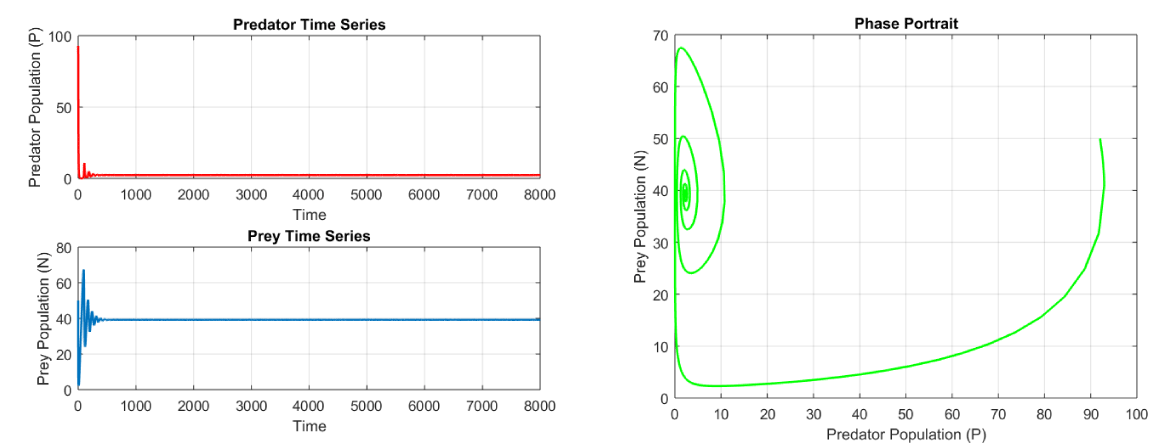
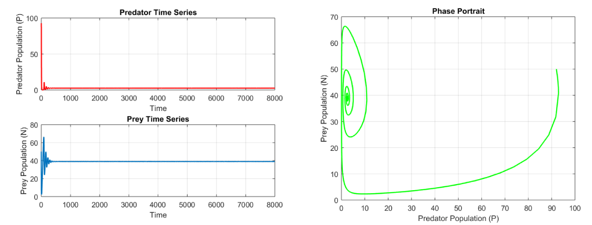
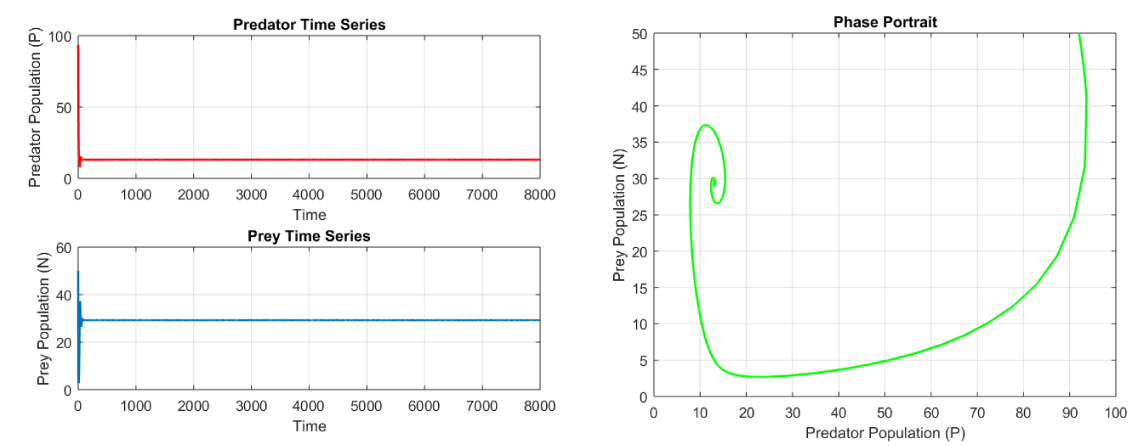
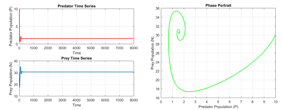
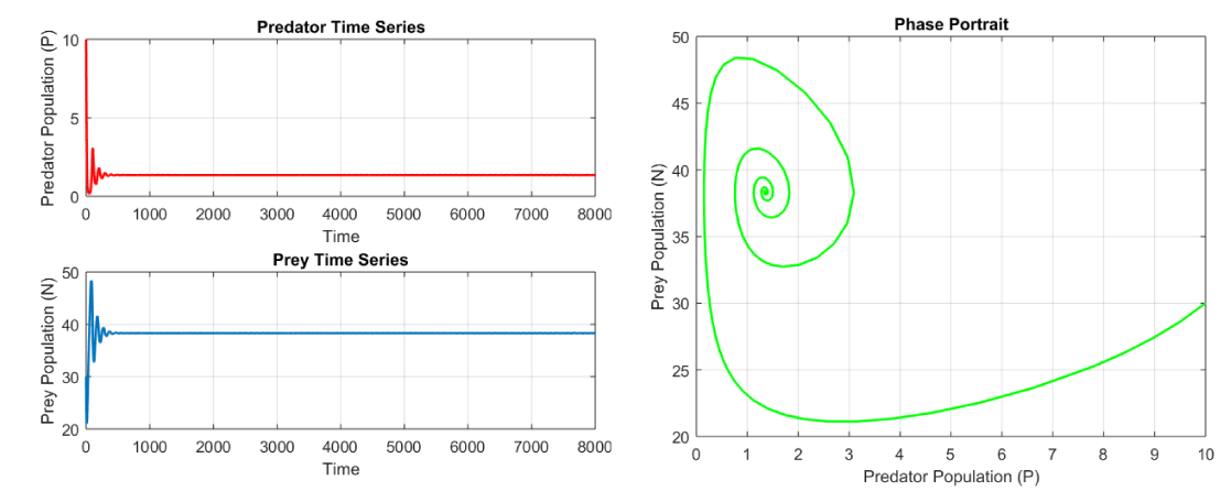
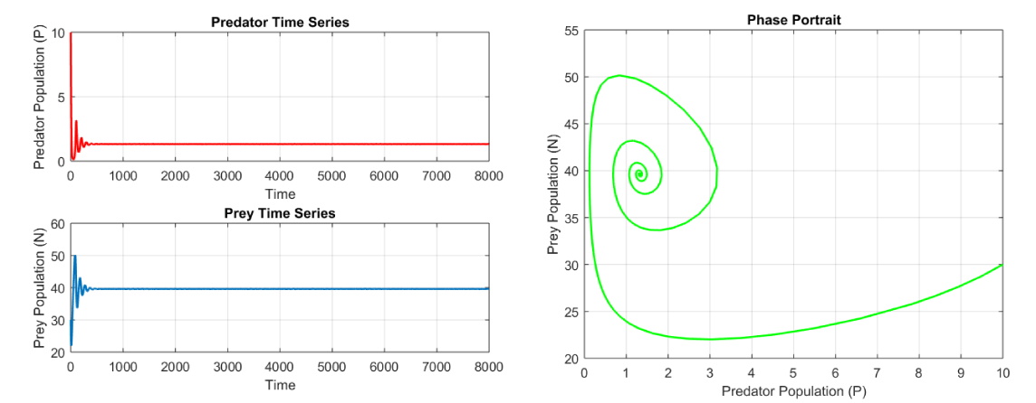
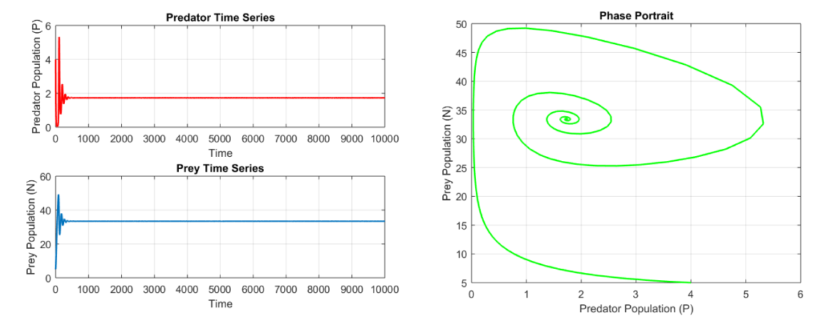
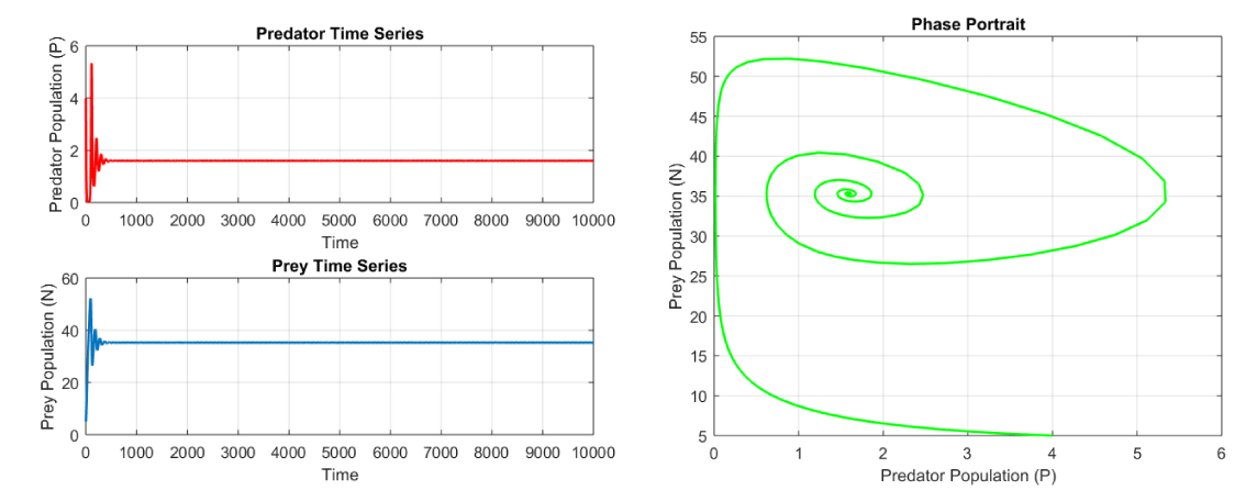
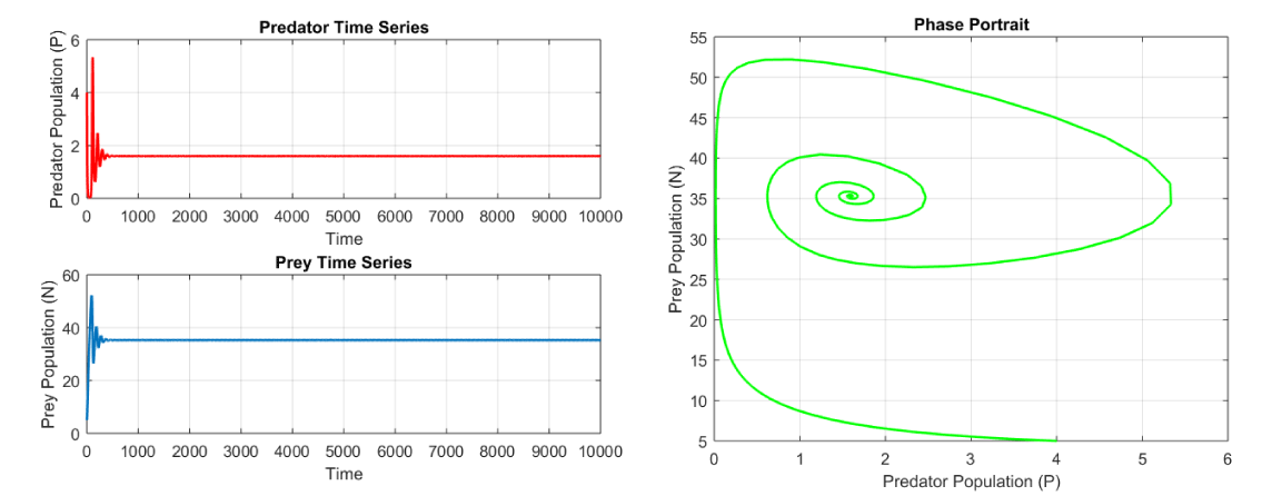
We present the effects of different parameters on the system (1-2) through plots. The phase portraits along with the time series solution are presented for different values of parameters. In the same section, we provide the analysis of results via Neural Networking.

Discussion

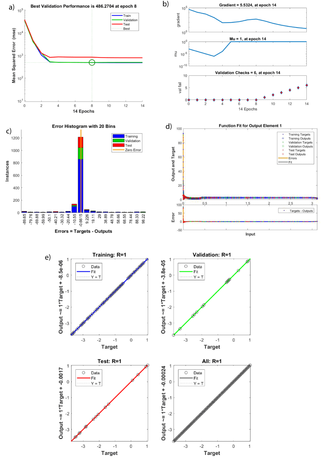
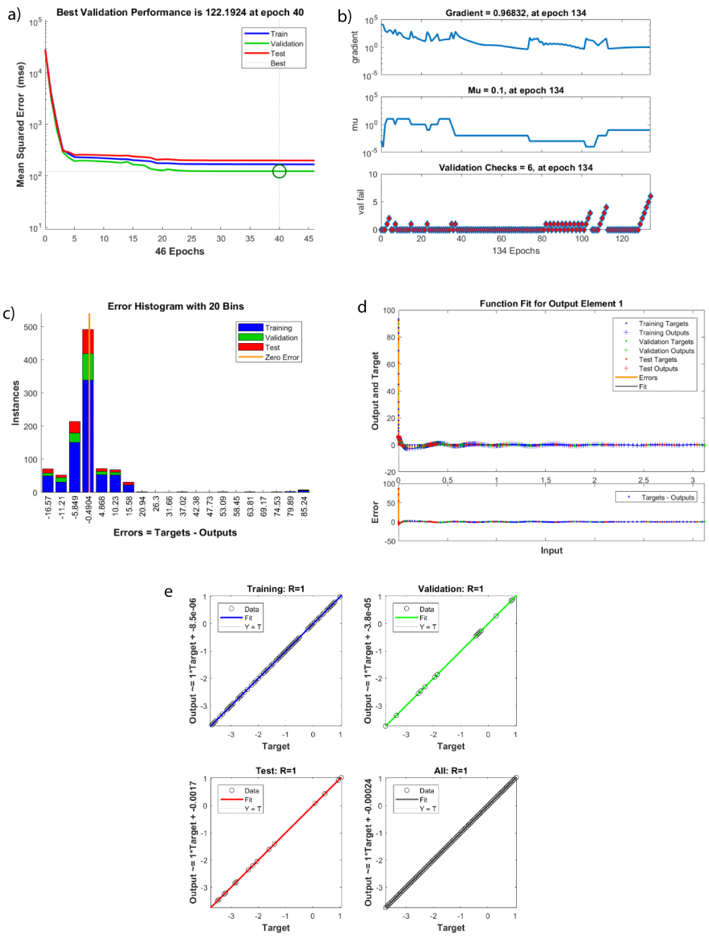
In Figure (2-4) the values of parameters are taken as a = 0.9, b = 0.79, α = 0.0092, m = 0.31, k = 0.071, dT = 10, s = 0.1 and n = 0.001. We have taken f = 0.9, 1.5 in plots 1, 2, and 3 respectively. Here P(0) = 92, N(0) = 50. The visual representations of plots offer a captivating insight into the complex dynamics of the predator-prey system, particularly emphasizing the pivotal role of the shared food resource, the prey's consumption rate, and the temperature differential. Observing Figures (2-4), it becomes evident that the predator population exhibits a pronounced positive response to an escalating value of f. This underscores the criticality of a plentiful food source in bolstering predator numbers. Such a correlation resonates with ecological principles, where the availability of resources directly influences population dynamics. In Figures (5-7) the values of parameters are taken as a = 0.73, b = 0.979, α = 0.0092, m = 0.31, k = 0.071, dT = 15, s = 0.01, n = 0.01 and f = 0.9. We have taken b = 0.179, 0.579, and 0.979 in plots 4, 5, and 6 respectively. Here P(0) = N(0) = 30. Delving into Plot (5-7), a compelling trend emerges: as the prey's consumption rate of f intensifies, so does its population. This direct relationship underscores the fundamental ecological tenet that enhanced consumption of resources fosters prey proliferation, leading to cascading effects up the trophic levels. In Figures (8-10) the values of parameters are taken as a = 0.73, b = 0.979, α = 0.0092, m = 0.31, k = 0.071, dT = 10, s = 0.71, n = 0.01 and f = 0.9. We have taken dT = 0, 10, and 20 in plots 7, 8, and 9 respectively. Here P(0) = 4, N(0) = 5. The most intriguing revelations come from Plots (8-10). As widens, a conspicuous surge in the predator population is observed. This can be attributed to thermoregulatory advantages conferred upon predators, enabling them to capitalize on temperature-driven ecological advantages. The escalating predator numbers in response to temperature gradients accentuate the intricate interplay between climate and predator-prey dynamics. In summation, these plots not only elucidate the multifaceted relationships within the predator-prey system but also underscore the profound impacts of environmental variables. They serve as a testament to the intricate ballet of nature, where subtle shifts in resources and climate can orchestrate significant changes in ecological dynamics. Figure 11(a) displays a Mean Squared Error (MSE) graph of a neural network-based prediction model for temperature difference 𝛿T. The model achieved its lowest MSE at epoch 8, with training performance generally lower than validation. Test performance is lower than training but higher than validation, indicating good generalization to unseen data. The model's performance is attributed to its low MSE on the validation set and its ability to generalize well to unseen data. The image highlights the model's accuracy and generalization capabilities. Figure 12(a) shows a graph of the best validation performance for a feed-forward neural network at each epoch. The performance increases rapidly in the early epochs, reaching a peak at 122.1924 at epoch 40. The training performance is always higher than the validation performance. Validation performance measures how well a model will perform on unseen data, calculated by evaluating the model on a separate dataset. The peak at epoch 40 is due to the model's best balance between underfitting and overfitting. Training performance is always higher than validation performance because the model is trained on training data.

Figure 2: Impact of food at f = 0.90.

Figure 3: Impact of food at f = 1.

Figure 4: Impact of food at f = 5.

Figure 5: Impact of food consumption rate at b = 0.179.

Figure 6: Impact of food consumption rate at b = 0.579.

Figure 7: Impact of food consumption rate at b =0.979.

Figure 8: Impact of temperature difference at δT = 0.

Figure 9: Impact of temperature difference at δT = 10.

Figure 10: Impact of temperature difference at δT = 20.

Figure 11: Visual Overview of Training Progress and Performance Metrics for Temperature Difference. (a). Results of MSE for case-1 (b). Results of transition case-1; (c). Error bar plot case-1 (d). Fitness plot case-1; (e). Regression illustration case-1

Figure 12: Visual Overview of Training Progress and Performance Metrics for Food. (a). Results of MSE case-2 (b). Results of transition case-2; (c). Error bar plot case-2 (d). Fitness plot case-2; (e). Regression illustration case-3

Figure 13: Visual Overview of Training Progress and Performance Metrics for Rate of food consumption by prey. (a). Results of MSE case-3 (b). Results of transition case-3' (c). Error bar plot case-3 (d). Fitness plot case-3; (e). Regression illustration case-3

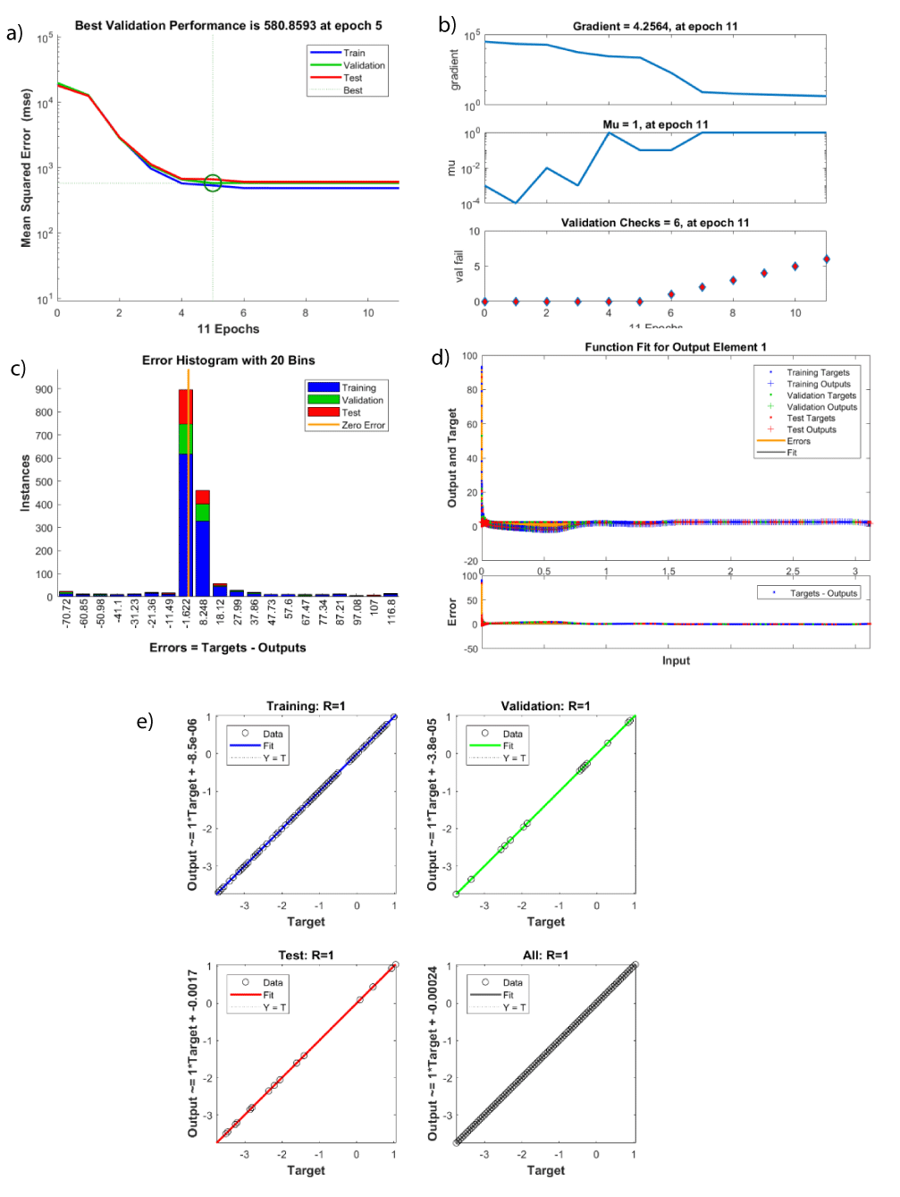
Figure 13 depicts a graph illustrating the training and validation performance of a machine learning model. The graph consists of four curves: blue, green, red, and purple. The training outputs closely follow the targets, indicating good learning. However, the validation outputs are not as closely following the targets, suggesting overfitting. The graph's "Best Validation Performance" is 550.8533 at epoch 5, indicating the model's best performance on validation data. The model's generalization is not good, suggesting further tuning or regularization. Figure 11(b) shows that the model is still learning at epoch 14, with a gradient of 5.5324 and validation checks of 6. The temperature difference T could impact the learning process, leading to the exploration of the parameter space and finding the global minimum. Lower temperature differences may lead to stable convergence but may prevent the model from finding the global minimum. The optimal temperature difference depends on the problem's complexity, data set size, and desired accuracy. Figure 12(b) shows a graph of a machine learning model's performance during training. It shows the gradient, validation checks, and epochs. The gradient starts high and gradually decreases as the model approaches optimal performance. The validation checks initially increase before fluctuating. The "val fail gradient" threshold is used to prevent overfitting by stopping the training process if the checks fall below a certain level. The model achieved a gradient of 5.5324 and a validation check score of 6 at epoch 14, with a learning rate of 1. Figure 13(b) shows a machine learning model's training and validation performance. The model maintains a constant number of validation checks and graduates, indicating learning and improving data classification. However, a gap between blue and green lines suggests a misclassification. The model's training outputs closely follow targets, indicating good learning, but validation outputs. Figure 12(c) illustrates the impact of temperature difference at 𝛿T on error histograms. The histogram shows the difference between predicted outputs and actual targets, with bins representing different error ranges. The training line has the most peaked errors, while the validation and test lines have less peaked ones. Overall, the temperature difference negatively impacts the neural network's performance. Figure 12(c) shows three graphs illustrating the performance of the machine learning model during training. The top graph shows the gradient, which indicates the model's learning rate, which starts high and gradually decreases as it approaches optimal performance. The middle graph tracks the model's performance on a separate data set, indicating its generalization beyond the training data. The bottom graph shows the val fail gradient, a threshold for validation checks, which stops the training process if the gradient falls below it. The text box displays the current values of the gradient, learning rate, and validation checks at epoch 14.

Figure 13(c) shows the training and validation results of a function, fitting a system. The model's training MSE decreases rapidly, indicating good learning, while the validation MSE overfits the training data. The test MSE is higher, indicating the model needs further tuning or regularization. Figures 11,12, and 13(d) illustrate the results of fitting a function to a system's output element 1, with training targets in blue, training outputs in green, validation targets in red, and validation outputs in purple, illustrating the system's performance. Figures 11,12,13(e) display the purposes of training, validation, and testing of the scenarios. The primary objective of this inquiry was to evaluate the accuracy of data prediction and forecasting. A regression result of R = 1 implies a high degree of correlation between the target and output variables throughout the computation.

Conclusion

Upon synthesizing the insights obtained from our thorough analysis, it becomes indisputable that the predator-prey system comprises complex inter-dependencies. This relationship is supported by the consumption rates, environmental temperature gradients, and the dynamics of a shared food resource. By employing modern computational techniques such as neural networks and rigorous mathematical analysis, our research has shed light on the significant consequences that resource abundance, consumption patterns, and climatic fluctuations have on ecological dynamics. The subtle equilibrium of natural systems is underscored by the undeniable positive correlation between f and predator proliferation, the direct influence of b on prey populations, and the nuanced response of predators to temperature gradients. The results of this study not only contribute to the advancement of knowledge regarding ecological principles but also emphasize the importance of comprehensive conservation approaches that acknowledge the complex interaction between biotic and abiotic elements. It is incumbent upon us, as custodians of the environment, to heed the advice contained within these analyses. The complex interaction between predators and prey, influenced by the patterns of resource availability and climatic fluctuations, serves as a powerful reminder of the resilience and vulnerability of nature. In this era of fast-paced environmental changes, the findings of this study urge us to adopt a mindset of sustainable coexistence. It emphasizes the need to achieve a harmonious relationship between different species and their environment, not only as a goal but as a shared necessity. Predator-prey interaction has been studied for many decades, but the complexity of the relationship opens a vast scope of research on this interaction. New trends like non-integer order models deal the complexity in a better way, in the future we shall look at the fractional-order model to study the complexity of the relationship.

1. Effati S, Mansoori A, Eshaghnezhad M, An efficient projection neural network for solving bilinear programming problems, Neurocomputing. 2015; 168:1188–1197.
2. Holling CS, The functional response of invertebrate predators to prey density, Mem. Entomol. Soc. Can. 1966; 98 (S48):5–86.
3. Biazar J, Montazeri R, A computational method for solution of the prey and predator problem, Appl. Math. Comput. 2005; 163 (2):841–847.
4. Solis FJ, Self-limitation in a discrete predator–prey model, Math. Comput. Modelling. 2008; 48(1):191–196.
5. Danca M, Codreanu S, Bakó B. Detailed analysis of a nonlinear prey-predator model. J Biol Phys. 1997 Mar; 23(1):11-20. doi: 10.1023/A:1004918920121. PMID: 23345647; PMCID: PMC3456267.
6. Jing Z, Yang J. Bifurcation and chaos in discrete-time predator–prey system, Chaos Solitons Fractals. 2006; 27(1): 259–277.
7. Liu X, Xiao D. Complex dynamic behaviors of a discrete-time predator–prey system, Chaos Solitons Fractals. 2007; 32(1):80–94.
8. Elsadany AEA, El-Metwally HA, Elabbasy EM, Agiza HN. Chaos and bifurcation of a nonlinear discrete prey-predator system, Comput. Ecol. Softw. 2012; 2(3):169.
9. Summers D, Cranford JG, Healey BP. Chaos in periodically forced discrete-time ecosystem models, Chaos Solitons Fractals. 2000; 11(14): 2331–2342.
10. Paul S, Mondal SP, Bhattacharya P, Numerical solution of Lotka Volterra prey predator model by using Runge–Kutta–Fehlberg method and Laplace Adomian decomposition method, Alex. Eng. J. 2016; 55(1):613–617.
11. Batiha B. The solution of the prey and predator problem by differential transformation method, Int. J. Basic Appl. Sci. 2014; 4(1):36–43.
12. Garvie MR, Burkardt J, Morgan J. Simple finite element methods for approximating predator-prey dynamics in two dimensions using MATLAB. Bull Math Biol. 2015 Mar; 77(3):548-78. doi: 10.1007/s11538-015-0062-z. Epub 2015 Jan 24. PMID: 25616741.
13. Bildik N, Deniz S. The use of Sumudu decomposition method for solving predator-prey systems, Math. Sci. Lett. 2016; 5(3):285–289.
14. Yu J, Yu J. Homotopy analysis method for a prey-predator system with Holling IV functional response, Appl. Mech. Mater. 2014.
15. Ray SS. A new coupled fractional reduced differential transform method for the numerical solution of fractional predator-prey system, CMES Comput. Model. Eng. Sci. 2015; 105(3).
16. Fang L, Wang J. The global stability and pattern formations of a predator–prey system with consuming resource. Applied Mathematics Letters. 2016; 58:49-55.
17. Ejaz A, Nawaz Y, Arif MS, Mashat DS, Abodayeh K. Stability Analysis of Predator-Prey System with Consuming Resource and Disease in Predator Species. CMES-Computer Modeling in Engineering & Sciences. 2022; 132(2).
18. Ejaz A, Nawaz Y, Arif MS, Mashat DS, Abodayeh K. Stability Analysis of Predator-Prey System with Consuming Resource and Disease in Predator Species. CMES-Computer Modeling in Engineering & Sciences. 2022; 132(2).
19. Arif MS, Abodayeh K, Ejaz A. Stability Analysis of Fractional-Order Predator-Prey System with Consuming Food Resource. Axioms. 2023; 12(1):64.
20. Mall S, Chakraverty S. Chebyshev Neural Network based model for solving Lane–Emden type equations, Appl. Math. Comput. 2014; 247:100–114.
21. Chakraverty S, Mall S. Regression-based weight generation algorithm in neural network for solution of initial and boundary value problems, Neural Comput. Appl. 2014; 25(3–4):585–594.
22. Raja MAZ, Samar R, Alaidarous ES, Shivanian E. Bio-inspired computing platform for reliable solution of Bratu-type equations arising in the modeling of electrically conducting solids. Appl Math Model. 2016; 40(11):5964-5977.
23. Raja MA, Zameer A, Khan AU, Wazwaz AM. A new numerical approach to solve Thomas-Fermi model of an atom using bio-inspired heuristics integrated with sequential quadratic programming. Springerplus. 2016 Aug 23; 5(1):1400. doi: 10.1186/s40064-016-3093-5. PMID: 27610319; PMCID: PMC4994819.
24. Effati S, Pakdaman M. Artificial neural network approach for solving fuzzy differential equations. Inform Sci. 2010; 180(8):1434-1457.
25. Raja MAZ. Solution of the one-dimensional Bratu equation arising in the fuel ignition model using ANN optimised with PSO and SQP. Connect Sci. 2014; 26(3):195-214.
26. Baymani M, Effati S, Niazmand H, Kerayechian A. Artificial neural network method for solving the Navier–Stokes equations. Neural Comput Appl. 2015; 26(4):765-773.
27. Raja MAZ, Ahmad I, Khan I, Syam MI, Wazwaz AM. Neuro-heuristic computational intelligence for solving nonlinear pantograph systems. Front Inf Technol Electron Eng. 2017; 18(4):464-484.
28. Effati S, Skandari MHN. Optimal control approach for solving linear Volterra integral equations. Int J Intell Syst Appl. 2012; 4(4):40.
29. Jafarian A, Measoomy S, Abbasbandy S. Artificial neural networks based modeling for solving Volterra integral equations system. Appl Soft Comput. 2015; 27:391-398.
30. Raja MAZ, Farooq U, Chaudhary NI, Wazwaz AM. Stochastic numerical solver for nanofluidic problems containing multi-walled carbon nanotubes. Appl Soft Comput. 2016; 38:561-586.
31. Effati S, Buzhabadi R. A neural network approach for solving Fredholm integral equations of the second kind. Neural Comput Appl. 2012; 21(5):843-852.
32. Ahmad I, Raja MAZ, Bilal M, Ashraf F. Neural network methods to solve the Lane–Emden type equations arising in thermodynamic studies of the spherical gas cloud model. Neural Comput Appl. 2017; 28(1):929-944. Available from: http://dx.doi.org/10.1007/s00521-016-2400-y
33. Raja MAZ, Khan JA, Chaudhary NI, Shivanian E. Reliable numerical treatment of nonlinear singular Flierl–Petviashivili equations for unbounded domain using ANN, GAs, and SQP. Appl Soft Comput. 2016; 38:617-636.
34. Sabouri J, Effati S, Pakdaman M. A neural network approach for solving a class of fractional optimal control problems. Neural Process Lett. 2016; (1-16).
35. Effati S, Mansoori A, Eshaghnezhad M. An efficient projection neural network for solving bilinear programming problems. Neurocomputing. 2015; 168:1188-1197.
36. Raja MAZ, Khan MAR, Mahmood T, Farooq U, Chaudhary NI. Design of bio-inspired computing technique for nanofluidics based on nonlinear Jeffery–Hamel flow equations. Can J Phys. 2016; 94(5):474-489.
37. Kumar M, Yadav N. Numerical solution of Bratu’s problem using multilayer perceptron neural network method. Nat Acad Sci Lett. 2015; 38(5):425-428.